Problem Statement & Motivation

In this first problem exploration, I will be using this video by TED-Ed as reference:

This video introduces the concept of Hotelling’s law; a game theory law which explains why two retailers selling the same product tend to set up shop close to each other.

I was motivated to make this simulation when I recently came across 2 cinemas situated side-by-side, and I decided to look up cinema locations within Singapore where I live. Lo and behold:

As you can see, cinemas tend to be isolated or clustered into pairs.

I decided to make a simple simulation of shops within a 2D space to see if I could reproduce this result. Python was used as the programming language.

Python notebook link (Google Colab)

The general idea was to randomly generate shop locations first, then have each shop shift its position little by little towards a more advantageous one. The metric used to determine the feasibility of a position was only the shop’s area of influence (as in the video), and other factors such as non-uniform population density and spatial obstacles were not considered for simplicity. The problem was restricted to a square domain of [0,1]×[0,1], wherein shops were not allowed to leave this domain and areas of influence were not allowed to exceed its boundaries.

Finding the Areas of Influence

Voronoi Diagrams

It was a simple task to randomly initialise points in a 2D domain, but it was immediately after that I came to realise my first problem: how do I calculate a shop’s area of influence? To be clear, a shop’s area of influence is defined as all points in the domain whereby the nearest shop is the one in question. Thankfully, there is a perfect solution for this problem: Voronoi diagrams.

A Voronoi diagram would partition the domain into regions, where each region corresponds to a shop’s area of influence. The scipy library provides a function to obtain the Voronoi diagram from a list of points. While I’m not familiar with the details of how it achieves this, it does so in $O(n\log{n})$ time for 2D points. Just when I thought I was done with this task, I plotted the diagram and noticed a glaring problem. Can you figure out what it is? (Hint: the lines describe the edges of the regions and the orange dots describe the vertices of the regions.)

Voronoi diagram of randomised 2D points (actual size)

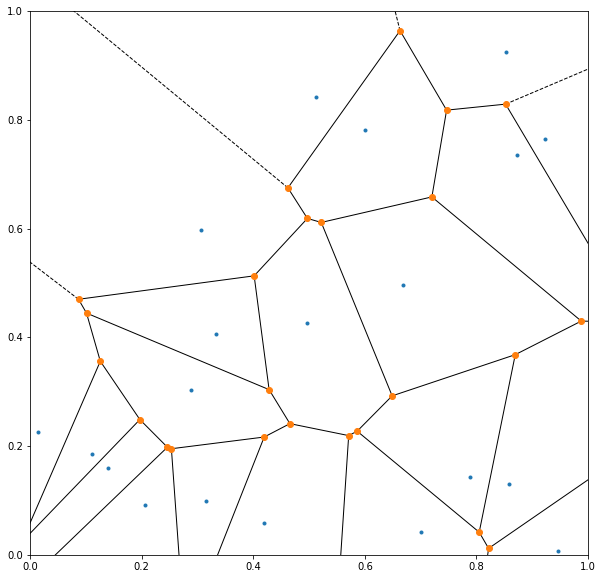
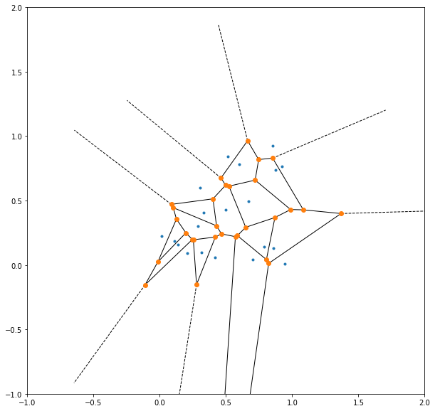
Now, it might not be immediately obvious from this image alone, but there is indeed a big problem: the diagram does not know what the problem domain is, and hence does not terminate at the boundary. This becomes evident when the diagram is zoomed out:

Voronoi diagram of randomised 2D points (zoomed out)

Reflection Augmentation

Unfortunately, scipy’s Voronoi class does not allow me to provide the domain boundary, which meant that I had to consult Google on how to implement bounded Voronoi diagrams. Not to anyone’s surprise, I found an answer on Stack Overflow. The trick was that, since the domain was rectangular, I could reflect the points off the left, right, top and bottom boundaries, and add those reflected points to my list of points. In doing so, all points outside the domain would be closest to a reflected point than one within the domain. Check it out:

Voronoi diagram of randomised 2D points (augmented. zoomed out)

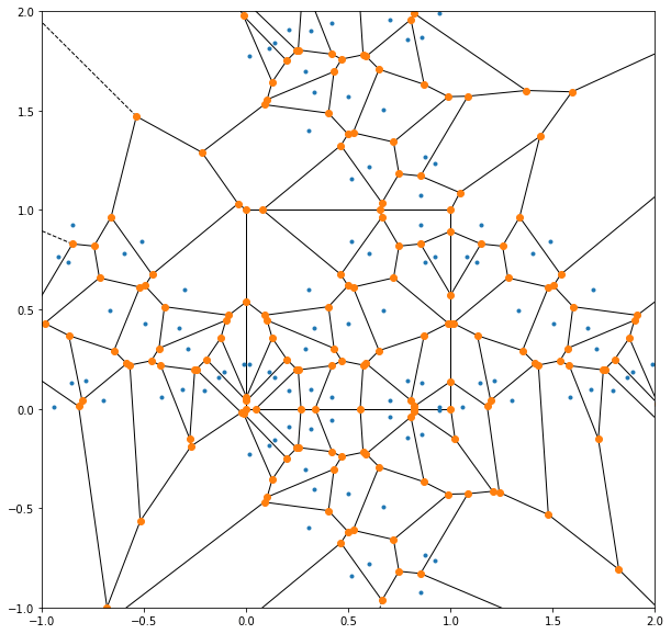
Notice here the edges forming a square where the boundary is supposed to be? This means that augmenting the list of points with the reflected points naturally leads to edges in the diagram inscribing the domain! This neat trick is so remarkable that it’s almost magical. Despite the additional computation cost incurred by increasing the number of points by 5 times, it certainly was a saner (and probably more efficient) option than manually calculating the edge-boundary intersections. I then only needed to select the regions within the domain.

Voronoi diagram of randomised 2D points (augmented, actual size)

There was only one step left to obtain the areas of influence, which was to calculate the area of a region given the coordinates of its vertices.

Convex Polygon Area

There is a well-known formula to obtain the area of a convex polygon given its coordinates in clockwise/anticlockwise order:

$A=\dfrac{1}{2}\begin{vmatrix}x_1 & y_1\\ x_2 & y_2\\ \vdots & \vdots\\ x_n & y_n\\ x_1 & y_1\end{vmatrix}\quad$

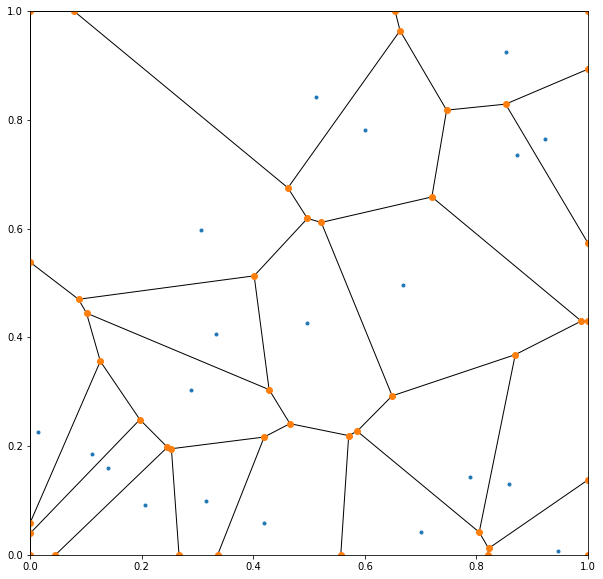
Using this formula, I calculated the area of each region and annotated each point with its relative area of influence, defined as the proportion of the current point’s area of influence compared to the average area of influence:

With this, the first obstacle is overcome and therewith the next: how do I know which direction and how far to shift the shops to reach a more advantageous position?

Maximising the Areas of Influence

Gradient Ascent

Warning: Lots of math ahead! As such, I will try to provide an explanation that does not rely on the formulae/equations involved.

In order to simulate a shop’s movement to a better location, I assumed every shop to behave according to the following rationale: At every time step, a shop will look around its current vicinity to determine the direction which increases its area of influence the most, and make a small movement towards that location. This was a simplified and unrealistic assumption since actual shops do not make smooth motions towards better locations, but nonetheless a good baseline to begin from.

Although there might be better algorithms to maximise each shop’s area of influence, I decided to stick to the simple algorithm of gradient ascent. The idea is that the gradient of the area of influence at some location points towards the direction of greatest increase. The gradient of a function in the Cartesian basis is simply:

$\nabla f(x,y)=\begin{pmatrix}\dfrac{\partial f}{\partial x}(x,y)\\\\\dfrac{\partial f}{\partial y}(x,y)\end{pmatrix}$

By making incremental steps in that direction with magnitude proportional to the gradient, every point will eventually reach a location with locally maximum area of influence:

$\begin{pmatrix}x\\y\end{pmatrix}_{n+1}=\begin{pmatrix}x\\y\end{pmatrix}_{n}+\alpha\nabla f(x_n,y_n)$

Of course, this brought to mind the issue of how the gradient could be computed numerically. There are 2 main methods used for numerical differentiation:

Automatic differentiation
Finite differencing

Note: Gradient ascent requires that the function be differentiable at every point in the domain, which does not hold if 2 off-centre points are extremely close to each other, as one point moving past the other would swap their areas of influence and thus cause a stepwise change. This will however give each pair of points the tendency to centralise itself.

Automatic Differentiation

Automatic differentiation is a powerful method that gives an exact value of the first derivative. The magic lies in introducing a special number $\epsilon$ , with the definition $\epsilon\ne0,\epsilon^2=0$ . Of course, $\epsilon$ itself is not a real/complex number since no such number would fulfil that definition. It is very similar to the complex unit $i$ , defined as $i\ne0,i^2=-1$ .

This technique can be easily understood by performing a Taylor series expansion on the function. Since all powers of $\epsilon$ greater than 2 are defined to be 0, they do not appear in the expansion:

$f(x+\epsilon,y)=f(x,y)+\dfrac{\partial f}{\partial x}(x,y)\epsilon$

$f(x,y+\epsilon)=f(x,y)+\dfrac{\partial f}{\partial y}(x,y)\epsilon$

The algorithmic implementation of this technique involves the use of dual numbers (a pair of numbers), typically defined as the function’s value and first derivative at a particular point. This dual number can be interpreted as the coefficient vector of $\epsilon$ . Numerical operations (addition, multiplication, etc.) have to be overridden to accommodate these dual numbers, which is difficult to implement with reflection augmentation. As such, I resorted to finite differencing, an approximate method.

Finite Differencing

Finite differencing is a straightforward technique which approximates the infinitesimals, $dx$ and $dy$ , with small but finite values, $\Delta x$ and $\Delta y$ . However, this also means that the derivative obtained through this technique is not exact. The accuracy can be improved by incorporating more points near where the derivative is to be calculated.

I used the central difference, defined as:

$\dfrac{\partial f}{\partial x}(x,y)=\dfrac{f(x+\Delta x,y)-f(x-\Delta x,y)}{2\Delta x}+O((\Delta x)^2)$

$\dfrac{\partial f}{\partial y}(x,y)=\dfrac{f(x,y+\Delta y)-f(x,y-\Delta y)}{2\Delta y}+O((\Delta y)^2)$

This basically meant that for every point, I had to bump it left, right, down and up a slight amount, and recalculate its area of influence on each bumped position. With those, I could calculate the partial derivatives and thereby the gradient.

Now that I had the means to calculate the gradient, I could finally begin running the simulation! One issue though, was that convergence could not be attained due to discontinuities in the gradient. Hence, I only ran the simulation for a fixed number of time steps.

Process Simulation

Pseudocode

The simulation process could be summarised into the following steps as discussed:

Randomly generate $n$ points in the 2D space.
Define finite steps $\Delta x$ and $\Delta y$ , as well as movement step size $\alpha$ .
Run simulation for time steps. At each time step:
1. Iterate across all points. At each point:
  1. Shift point left and right by $\Delta x$ , and up and down by $\Delta y$ , calculating the new area of influence at each position.
  2. Calculate the gradient of the area of influence using the central difference method.
  3. Scale the gradient by $\alpha$ and add the result to the point’s original position.
  4. If the point exits the domain, shift it back to its original position.

For the programming-inclined, this has a time complexity of $O(kn^2\log{n})$ .

Results

For these examples, I set $\Delta x=\Delta y=0.001$ , $\alpha=0.01$ , and ran the simulations for 1000 time steps.

Two Points

Due to the heavy dependence of the time complexity on the number of points, I decided to start with the simple case of 2 points, just like in the TED-Ed video:

After running the simulation, they converged to the following result:

data:image/png;base64,iVBORw0KGgoAAAANSUhEUgAAAlsAAAJDCAYAAAA8QNGHAAAABHNCSVQICAgIfAhkiAAAAAlwSFlzAAALEgAACxIB0t1+/AAAADh0RVh0U29mdHdhcmUAbWF0cGxvdGxpYiB2ZXJzaW9uMy4xLjEsIGh0dHA6Ly9tYXRwbG90bGliLm9yZy8QZhcZAAAbfElEQVR4nO3df7BdZX3v8c83CT/sVbFCmYYkRbxBphgyIFG4tWO11JYwnTCd3muh1+FSnMYytXgVa7V2aEtnbu1PWttYG7UVdAo3pdamrUhnkKrtGAqpmopok+FHk5iRooBXRQF57h/nGAOGZBPO95yc8HrNZObsvZ691rNnzTl5n7X2WavGGAEAoMeCuZ4AAMChTGwBADQSWwAAjcQWAEAjsQUA0EhsAQA02m9sVdWfVdXdVfXpx1leVfW2qtpWVVuq6gUzP00AgPlpkiNb70ly9j6Wr05y4vS/tUn+5MlPCwDg0LDf2BpjfDTJl/Yx5NwkV40pm5I8q6oWz9QEAQDms5n4zNaSJNv3eLxj+jkAgKe8RbO5sapam6lTjTn6aTn9Oc/6dutt3vXIbE4FAGCfTl/87U65875Hcs/XRh3IemYitnYmWbbH46XTz32HMcb6JOuTZNVxC8cta58+teCoZcnr9vr5ewCAuXHFiuT+qZN3q9Z/5YBXMxOnETcmuWD6rxLPTHL/GGPXxK8+7GnJWZfNwDQAAGbQWZdNdcqTtN8jW1V1dZKXJjmmqnYk+dUkhyXJGOMdST6Y5Jwk25J8LcnPTLz1o5ZNvZGVr3jCEwcAaPWtPrnh8iS3HfBqaowxMxN6ohuuGnO1bQCAJ6KqNo8xVh3Ia11BHgCgkdgCAGgktgAAGoktAIBGYgsAoJHYAgBoJLYAABqJLQCARmILAKCR2AIAaCS2AAAaiS0AgEZiCwCgkdgCAGgktgAAGoktAIBGYgsAoJHYAgBoJLYAABqJLQCARmILAKCR2AIAaCS2AAAaiS0AgEZiCwCgkdgCAGgktgAAGoktAIBGYgsAoJHYAgBoJLYAABqJLQCARmILAKCR2AIAaCS2AAAaiS0AgEZiCwCgkdgCAGgktgAAGoktAIBGYgsAoJHYAgBoJLYAABqJLQCARmILAKCR2AIAaCS2AAAaiS0AgEZiCwCgkdgCAGgktgAAGoktAIBGYgsAoJHYAgBoJLYAABqJLQCARmILAKCR2AIAaCS2AAAaiS0AgEZiCwCgkdgCAGgktgAAGoktAIBGYgsAoJHYAgBoJLYAABqJLQCARmILAKCR2AIAaCS2AAAaiS0AgEZiCwCgkdgCAGgktgAAGoktAIBGYgsAoJHYAgBoJLYAABqJLQCARmILAKCR2AIAaCS2AAAaiS0AgEZiCwCgkdgCAGgktgAAGoktAIBGYgsAoJHYAgBoJLYAABqJLQCARmILAKCR2AIAaCS2AAAaiS0AgEZiCwCgkdgCAGgktgAAGoktAIBGE8VWVZ1dVZ+rqm1V9aa9LP++qrqxqj5RVVuq6pyZnyoAwPyz39iqqoVJ1iVZneTkJOdX1cmPGfYrSTaMMU5Lcl6St8/0RAEA5qNJjmy9KMm2McbtY4wHk1yT5NzHjBlJnjn99VFJPj9zUwQAmL8WTTBmSZLtezzekeSMx4z5tST/UFW/kOS/JPmRGZkdAMA8N1MfkD8/yXvGGEuTnJPkvVX1HeuuqrVVdUtV3TJD2wUAOKhNEls7kyzb4/HS6ef29KokG5JkjPHxJEcmOeaxKxpjrB9jrBpjrDqw6QIAzC+TxNbNSU6sqhOq6vBMfQB+42PG/EeSs5Kkqr4/U7H1nzM5UQCA+Wi/sTXGeDjJa5Jcn+S2TP3V4a1VdXlVrZkedmmSn62qTyW5OsmFY4zRNWkAgPmi5qqJqkqPAQDzQlVtPtCPQbmCPABAI7EFANBIbAEANBJbAACNxBYAQCOxBQDQSGwBADQSWwAAjcQWAEAjsQUA0EhsAQA0ElsAAI3EFgBAI7EFANBIbAEANBJbAACNxBYAQCOxBQDQSGwBADQSWwAAjcQWAEAjsQUA0EhsAQA0ElsAAI3EFgBAI7EFANBIbAEANBJbAACNxBYAQCOxBQDQSGwBADQSWwAAjcQWAEAjsQUA0EhsAQA0ElsAAI3EFgBAI7EFANBIbAEANBJbAACNxBYAQCOxBQDQSGwBADQSWwAAjcQWAEAjsQUA0EhsAQA0ElsAAI3EFgBAI7EFANBIbAEANBJbAACNxBYAQCOxBQDQSGwBADQSWwAAjcQWAEAjsQUA0EhsAQA0ElsAAI3EFgBAI7EFANBIbAEANBJbAACNxBYAQCOxBQDQSGwBADQSWwAAjcQWAEAjsQUA0EhsAQA0ElsAAI3EFgBAI7EFANBIbAEANBJbAACNxBYAQCOxBQDQSGwBADQSWwAAjcQWAEAjsQUA0EhsAQA0ElsAAI3EFgBAI7EFANBIbAEANBJbAACNxBYAQCOxBQDQSGwBADQSWwAAjcQWAEAjsQUA0EhsAQA0ElsAAI3EFgBAI7EFANBIbAEANBJbAACNJoqtqjq7qj5XVduq6k2PM+YVVfWZqrq1qv5iZqcJADA/LdrfgKpamGRdkpcn2ZHk5qraOMb4zB5jTkzy5iQvHmPcW1XHdk0YAGA+meTI1ouSbBtj3D7GeDDJNUnOfcyYn02yboxxb5KMMe6e2WkCAMxPk8TWkiTb93i8Y/q5PT0vyfOq6p+ralNVnT1TEwQAmM/2exrxCaznxCQvTbI0yUer6pQxxn17DqqqtUnWztA2AQAOepMc2dqZZNkej5dOP7enHUk2jjEeGmPckeTfMxVfjzLGWD/GWDXGWHWgEwYAmE8mia2bk5xYVSdU1eFJzkuy8TFjPpCpo1qpqmMydVrx9hmcJwDAvLTf2BpjPJzkNUmuT3Jbkg1jjFur6vKqWjM97PokX6yqzyS5MckvjjG+2DVpAID5osYYc7PhqjFX2wYAeCKqavOBfgzKFeQBABqJLQCARmILAKCR2AIAaCS2AAAaiS0AgEZiCwCgkdgCAGgktgAAGoktAIBGYgsAoJHYAgBoJLYAABqJLQCARmILAKCR2AIAaCS2AAAaiS0AgEZiCwCgkdgCAGgktgAAGoktAIBGYgsAoJHYAgBoJLYAABqJLQCARmILAKCR2AIAaCS2AAAaiS0AgEZiCwCgkdgCAGgktgAAGoktAIBGYgsAoJHYAgBoJLYAABqJLQCARmILAKCR2AIAaCS2AAAaiS0AgEZiCwCgkdgCDjkXXXRRjj322KxYsWKvy8cYueSSS7J8+fKsXLky//qv/5okueuuu/KCF7wgp556ap7//OfnHe94x+7XbN68OaecckqWL1+eSy65JGOMWXkvwPwntoBDzoUXXpgPfehDj7v8uuuuy9atW7N169asX78+F198cZJk8eLF+fjHP55PfvKTuemmm/LWt741n//855MkF198cd75znfuft2+1g+wJ7EFHHJe8pKX5NnPfvbjLv+bv/mbXHDBBamqnHnmmbnvvvuya9euHH744TniiCOSJN/4xjfyyCOPJEl27dqVL3/5yznzzDNTVbngggvygQ98YFbeCzD/iS3gKWfnzp1ZtmzZ7sdLly7Nzp07kyTbt2/PypUrs2zZsvzSL/1SjjvuuOzcuTNLly7d63iA/RFbAHtYtmxZtmzZkm3btuXKK6/MF77whbmeEjDPiS3gKWfJkiXZvn377sc7duzIkiVLHjXmuOOOy4oVK/Kxj30sS5YsyY4dO/Y5HuDxiC3gkLH5rnuz7sZt2XzXvfsct2bNmlx11VUZY2TTpk056qijsnjx4uzYsSMPPPBAkuTee+/NP/3TP+Wkk07K4sWL88xnPjObNm3KGCNXXXVVzj333Nl4S8AhYNFcTwBgJmy+6978z3dtyoMPP5J7Nv5ODv/Pz+b+e7+YpUuX5td//dfz0EMPJUl+7ud+Luecc04++MEPZvny5fmu7/qu/Pmf/3mS5Lbbbsull16aqsoYI294wxtyyimnJEne/va358ILL8wDDzyQ1atXZ/Xq1XP2XoH5pebqWjFVNVynBpgp627clt/7h8/lkZEsrOT1P3pSfv5ly+d6WsAhoqo2jzFWHchrnUYEDglnPvfoHL5oQRZWctiiBTnzuUfP9ZQAkjiyBRxCNt91bzbd/sWc+dyjc/rx3z3X0wEOIfPyyNbpixckV6xItmyYqykAh5jTj//u/PzLlgstYOZs2ZBcsSKnL15w+oGuYm5PI96/PfnbSwQXMOM+9KEP5aSTTsry5cvz1re+9TuW33XXXTnrrLOycuXKvPSlL919aYcbb7wxp5566u5/Rx555O6rxd9xxx0544wzsnz58vzUT/1UHnzwwVl9T8As27JhqlPu377/sfswZ6cRVx23cNyy9ulJki98/fC8cvOp355UVevXs7EN27Zt2567bY8x8su//Mu59NJL8+xnPzuXX355Xv3qVz/qKvDr1q3Lqaeemh/8wR/Mbbfdlo997GN59atf/ah1ffWrX80b3vCG/OEf/mGOPPLIvO1tb8sLX/jC/MAP/EDe/e535/jjj8/LX/7yg+Z927Zt2/bMfn3kO16YBV+e+kVs1fqv5JbPf/PRk5nQQXHph2OPfChvfOMbk0z9kPyWjq9nYxu2bduPt+xbj59q73u2t3333XfnsMMOy2c/+9kkybHHHpu//uu/3n0ZhzFGtm7dmuOPPz433HBDxhi5+eab89znPvdR69m6dWu+53u+Jx/+8IczxsinPvWpnHDCCfm7v/u7LFy4MNddd93u63IdDO/btm3btmf266++8bCkDqivHuWgiK06aul3/HYIcKCuvfbafO/3fm/e9a53JUne+9735qabbsof//Ef7x7z0z/90znjjDPy2te+Nu9///vzvve9L3/wB3+Qo4/+9l8x/vAP/3D+6I/+KD/+4z+ee+65J//yL/+Sa665JsnUPRRXr16dq6++enbfHDB7rljxpE8hJnP9ma0kOexpyVmXzfUsgKeY3/3d381HPvKRnHbaafnIRz6SJUuWZOHChbuX79q1K//2b/+WH/uxH5vDWQJz6qzLpjrlSZrbI1tHLZt6IytfMafTAA4tk9778P3vf3+S5Ctf+Ur+6q/+Ks961rN2L9+wYUN+4id+IocddliS5Oijj859992Xhx9+OIsWLXJ/RHgq+Faf3HB5ktsOeDVzdmRr865Hktd9WmgBM+Zb90ZccOzybN26NXfccUcefPDBXHPNNVmzZs2jxt5zzz155JFHkiS/+Zu/mYsuuuhRy6+++uqcf/75ux9XVV72spfl2muvTZJceeWV7o8ITwUrX5G87tPZvOuRzQe6Chc1BQ4Je94b8fBFC3Lxf/1/Wfd/fiXf/OY3c9FFF+Utb3lLLrvssqxatSpr1qzJtddemze/+c2pqrzkJS/JunXrcsQRRyRJ7rzzzrz4xS/O9u3bs2DBt38nvf3223PeeeflS1/6Uk477bS8733v2/0a4NBWT+KipmILOCS4NyLQ6cnE1tx/QB5gBrg3InCwcmQLOGS4NyLQxWlEAIBGTiMCABykxBYAQCOxBQDQSGwBADQSWwAAjcQWAEAjsQUA0EhsAQA0ElsAAI3EFgBAI7EFANBIbAEANBJbAACNxBYAQCOxBQDQSGwBADQSWwAAjcQWAEAjsQUA0EhsAQA0ElsAAI3EFgBAI7EFANBIbAEANBJbAACNxBYAQCOxBQDQSGwBADQSWwAAjcQWAEAjsQUA0EhsAQA0mii2qursqvpcVW2rqjftY9xPVtWoqlUzN0UAgPlrv7FVVQuTrEuyOsnJSc6vqpP3Mu4ZSV6b5KaZniQAwHw1yZGtFyXZNsa4fYzxYJJrkpy7l3G/keS3knx9BucHADCvTRJbS5Js3+PxjunndquqFyRZNsb4+xmcGwDAvLfoya6gqhYk+f0kF04wdm2StU92mwAA88UkR7Z2Jlm2x+Ol0899yzOSrEjyj1V1Z5Izk2zc24fkxxjrxxirxhg+QA8APCVMEls3Jzmxqk6oqsOTnJdk47cWjjHuH2McM8Z4zhjjOUk2JVkzxrilZcYAAPPIfmNrjPFwktckuT7JbUk2jDFurarLq2pN9wQBAOazGmPMzYarxlxtGwDgiaiqzQf6MShXkAcAaCS2AAAaiS0AgEZiCwCgkdgCAGgktgAAGoktAIBGYgsAoJHYAgBoJLYAABqJLQCARmILAKCR2AIAaCS2AAAaiS0AgEZiCwCgkdgCAGgktgAAGoktAIBGYgsAoJHYAgBoJLYAABqJLQCARmILAKCR2AIAaCS2AAAaiS0AgEZiCwCgkdgCAGgktgAAGoktAIBGYgsAoJHYAgBoJLYAABqJLQCARmILAKCR2AIAaCS2AAAaiS0AgEZiCwCgkdgCAGgktgAAGoktAIBGYgsAoJHYAgBoJLYAABqJLQCARmILAKCR2AIAaCS2AAAaiS0AgEZiCwCgkdgCAGgktgAAGoktAIBGYgsAoJHYAgBoJLYAABqJLQCARmILAKCR2AIAaCS2AAAaiS0AgEZiCwCgkdgCAGgktgAAGoktAIBGYgsAoJHYAgBoJLYAABqJLQCARmILAKCR2AIAaCS2AAAaiS0AgEZiCwCgkdgCAGgktgAAGoktAIBGYgsAoJHYAgBoJLYAABqJLQCARmILAKCR2AIAaCS2AAAaiS0AgEZiCwCgkdgCAGgktgAAGoktAIBGYgsAoJHYAgBoJLYAABqJLQCARmILAKCR2AIAaCS2AAAaiS0AgEZiCwCg0USxVVVnV9XnqmpbVb1pL8tfX1WfqaotVXVDVR0/81MFAJh/9htbVbUwybokq5OcnOT8qjr5McM+kWTVGGNlkmuT/PZMTxQAYD6a5MjWi5JsG2PcPsZ4MMk1Sc7dc8AY48YxxtemH25KsnRmpwkAMD9NEltLkmzf4/GO6ecez6uSXPdkJgUAcKhYNJMrq6pXJlmV5IceZ/naJGtncpsAAAezSWJrZ5JlezxeOv3co1TVjyR5S5IfGmN8Y28rGmOsT7J+evx4wrMFAJhnJjmNeHOSE6vqhKo6PMl5STbuOaCqTkvyp0nWjDHunvlpAgDMT/uNrTHGw0lek+T6JLcl2TDGuLWqLq+qNdPDfifJ05P8ZVV9sqo2Ps7qAACeUmqMuTmbV1VjrrYNAPBEVNXmMcaqA3mtK8gDADQSWwAAjcQWAEAjsQUA0EhsAQA0ElsAAI3EFgBAI7EFANBIbAEANBJbAACNxBYAQCOxBQDQSGwBADQSWwAAjcQWAEAjsQUA0EhsAQA0ElsAAI3EFgBAI7EFANBIbAEANBJbAACNxBYAQCOxBQDQSGwBADQSWwAAjcQWAEAjsQUA0EhsAQA0ElsAAI3EFgBAI7EFANBIbAEANBJbAACNxBYAQCOxBQDQSGwBADQSWwAAjcQWAEAjsQUA0EhsAQA0ElsAAI3EFgBAI7EFANBIbAEANBJbAACNxBYAQCOxBQDQSGwBADQSWwAAjcQWAEAjsQUA0EhsAQA0ElsAAI3EFgBAI7EFANBIbAEANBJbAACNxBYAQCOxBQDQSGwBADQSWwAAjcQWAEAjsQUA0EhsAQA0ElsAAI3EFgBAI7EFANBIbAEANBJbAACNxBYAQCOxBQDQSGwBADQSWwAAjcQWAEAjsQUA0EhsAQA0ElsAAI3EFgBAI7EFANBIbAEANBJbAACNxBYAQCOxBQDQSGwBADQSWwAAjcQWAEAjsQUA0EhsAQA0ElsAAI3EFgBAI7EFANBIbAEANBJbAACNxBYAQCOxBQDQSGwBADQSWwAAjcQWAEAjsQUA0Gii2Kqqs6vqc1W1raretJflR1TV/51eflNVPWemJwoAMB/tN7aqamGSdUlWJzk5yflVdfJjhr0qyb1jjOVJrkjyW/tb7+mLFyRXrEi2bHjiswYAmA1bNiRXrMjpixecfqCrmOTI1ouSbBtj3D7GeDDJNUnOfcyYc5NcOf31tUnOqqra75rv35787SWCCwA4+GzZMNUp929/UquZJLaWJNlzKzumn9vrmDHGw0nuT3L0RDN46IHkhssnGgoAMGtuuHyqU56kRTMwlYlV1doka5Pk6Kclq9Z/ZXrJbdn8+to8m3PhSTsmyT1zPQkOiH03v9l/85d9N8/seerwzvseOeD1TBJbO5Ms2+Px0unn9jZmR1UtSnJUki8+dkVjjPVJ1idJVd1yz9e+uepAJs3cq6pbxhj23zxk381v9t/8Zd/Nb1V1y4G+dpLTiDcnObGqTqiqw5Ocl2TjY8ZsTPK/pr/+70k+PMYYBzopAIBDxX6PbI0xHq6q1yS5PsnCJH82xri1qi5PcssYY2OSdyd5b1VtS/KlTAUZAMBT3kSf2RpjfDDJBx/z3GV7fP31JP/jCW57/RMcz8HF/pu/7Lv5zf6bv+y7+e2A91852wcA0MftegAAGrXHllv9zF8T7LvXV9VnqmpLVd1QVcfPxTzZu/3tvz3G/WRVjaryV1IHkUn2X1W9Yvp78Naq+ovZniN7N8HPzu+rqhur6hPTPz/PmYt58p2q6s+q6u6q+vTjLK+qetv0vt1SVS+YZL2tsdV1qx/6TbjvPpFk1RhjZabuHPDbsztLHs+E+y9V9Ywkr01y0+zOkH2ZZP9V1YlJ3pzkxWOM5yf537M+Ub7DhN97v5JkwxjjtEz9QdnbZ3eW7MN7kpy9j+Wrk5w4/W9tkj+ZZKXdR7b6bvVDt/3uuzHGjWOMr00/3JSpa7BxcJjkey9JfiNTv+B8fTYnx35Nsv9+Nsm6Mca9STLGuHuW58jeTbLvRpJnTn99VJLPz+L82IcxxkczdVWFx3NukqvGlE1JnlVVi/e33u7Y6r3VD50m2Xd7elWS61pnxBOx3/03ffh72Rjj72dzYkxkku+/5yV5XlX9c1Vtqqp9/TbO7Jlk3/1akldW1Y5M/aX/L8zO1JgBT/T/xiSzfLseDk1V9cokq5L80FzPhclU1YIkv5/kwjmeCgduUaZOZbw0U0eVP1pVp4wx7pvTWTGJ85O8Z4zxe1X13zJ1ncoVY4wDvx8MB7XuI1tP5FY/2detfph1k+y7VNWPJHlLkjVjjG/M0tzYv/3tv2ckWZHkH6vqziRnJtnoQ/IHjUm+/3Yk2TjGeGiMcUeSf89UfDG3Jtl3r0qyIUnGGB9PcmSm7pvIwW+i/xsfqzu23Opn/trvvquq05L8aaZCy+dFDi773H9jjPvHGMeMMZ4zxnhOpj5zt2aMccD3/mJGTfKz8wOZOqqVqjomU6cVb5/NSbJXk+y7/0hyVpJU1fdnKrb+c1ZnyYHamOSC6b9KPDPJ/WOMXft7UetpRLf6mb8m3He/k+TpSf5y+m8a/mOMsWbOJs1uE+4/DlIT7r/rk/xoVX0myTeT/OIYw1mBOTbhvrs0yTur6nWZ+rD8hQ4yHByq6upM/RJzzPRn6n41yWFJMsZ4R6Y+Y3dOkm1JvpbkZyZar/0LANDHFeQBABqJLQCARmILAKCR2AIAaCS2AAAaiS0AgEZiCwCgkdgCAGj0/wEsSh8JB2jI2AAAAABJRU5ErkJggg== — 2-point simulation (converged state)

The result agrees with Hotelling’s law, which is great.

Three Points

I then ran the simulation again with an additional point, and obtained the following result:

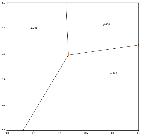
This was a bemusing result, as it seems like the point on the left could improve its own position by shifting towards the right. Perhaps there was an error with my program, or just that it was already a local minimum for that point. Either way, I might revisit this in the future.

Many Points

Of course, it seemed necessary that I should run this for many points, which I did. Here are the results for 20 points:

This result shows that points have a tendency to remain isolated or pair up with another point. Running the simulation several times with different initial conditions led to the same phenomenon. Isn’t it satisfying how similar this is to the distribution of cinemas in Singapore?

Conclusion & Further Ideas

This simulation generated rather interesting results, which provide an idea of what would happen when the concept behind Hotelling’s law is applied to many points. As mentioned, this was a very simplified simulation, yet it still took a considerable amount of time to run (about 2 minutes for 20 points). The simulation process might not have accurately modelled a realistic situation, but the results were still close.

In the future, I might consider making the following improvements:

Make shops relocate discontinuously instead of smoothly.
Model the business folding process whereby a shop would close down if its influence remains too low for an extended amount of time.

Further suggestions are welcome!