Probability Theory with Linear Algebra

This post was inspired by a MathOverflow problem: Coin flipping and a recurrence relation.

Let’s start by taking a look at an interesting problem from probability theory. We have 6 biased coins, each with 2 sides: heads and tails. The probability of a coin landing on heads is given as $p$ . Assume that initially, we only have tails facing up for all 6 coins.

$\left\{\text{T,T,T,T,T,T}\right\}$

On every time step, we take all the coins with tails facing up, and we flip them. If a coin lands on head, we do not flip it over again. The goal is to get heads facing up for all coins. The question is: if we repeat this entire process many times, how many time steps do we have to wait on average for all the coins to end up on heads?

representing the coins’ state

Let’s first think about how many possible states our coins can be in. Firstly, let’s notice that it does not matter how the coins are ordered. For example, the two states below are equal:

$\left\{\text{T,T,T,H,H,H}\right\} = \left\{\text{T,H,T,H,T,H}\right\}$

In combinatorics, in order to count the number of states when there are multiple objects, we first need to identify the nature of the setup:

	Permutation	Combination
No Repetition	Ordering with no identical objects. e.g. Ordering 6 different-coloured balls in a line.	Selection with no identical objects e.g. Selecting 2 out of 6 unique balls.
Repetition	Ordering with some identical objects e.g. Ordering 3 red balls and 3 blue balls in a line.	Selection with some identical objects e.g. Placing 6 identical balls into 2 unique slots.

Identifying the setup is useful because it gives us a standardised way to calculate the total number of states. This problem is straightforward enough for us to see that since the number of heads/tails range from 0 to 6 (both inclusive), there are 7 states in total. However, we will follow through with the calculation nonetheless.

In this problem, we essentially have 6 identical coins, with 2 unique slots: heads and tails. Hence, what we have here is combination with repetition. For placing $r$ objects into $n$ slots, the total number of states $\left|S\right|$ can be calculated as:

$\left|S\right|={n+r-1\choose r}$

For our problem, the number of states is ${2+6-1\choose 6}=7$ , which agrees with our observation from earlier. For this problem, we shall take the state to be the number of heads. We have the following states in our problem (our state space):

$S=\left\{0,1,2,3,4,5,6\right\}$

This means that we start from state 0, and our goal is to reach state 6.

the classic way

There are a few approaches to this problem. Let’s first try applying classical probability theory. This approach requires a strong intuition for probability, and this problem is not straightforward to analyse. We shall denote the expected number of steps needed to make r coins land on heads as $\mathbb{E}[T_r]$ .

Let us start with the simple case of only 1 coin, and build our solution up to 6 coins. For 1 coin, notice that on the first throw, there are 2 possibilities:

With a probability of $p$ , the coin lands on heads, and we don’t need to flip the coin any more.
With a probability of $(1-p)$ , the coin lands on tails, and we can expect to flip the coin $\mathbb{E}[T_1]$ more times before it lands on heads.

Our probability tree diagram looks like this:

Hence, the expected time for 1 coin to land on heads is:

$\mathbb{E}\left[T_1\right]=1+p\cdot 0+(1-p)\cdot\mathbb{E}\left[T_1\right]$

We have a recurrence relation here, and we can solve this by moving the terms with $\mathbb{E}\left[T_1\right]$ to the left side and diving both sides by the coefficient:

$\mathbb{E}\left[T_1\right]=\dfrac{1}{1-(1-p)}$

Now, let’s look at the case of 2 coins. Now, on the first throw, there are 4 possibilities:

With a probability of $p^2$ , the coins land on heads, heads, and we don’t need to flip the coins any more.
With a probability of $p(1-p)$ , the coins land on heads, tails, and we can expect to flip the coin $\mathbb{E}[T_1]$ more times before it lands on heads.
With a probability of $p(1-p)$ , the coins land on tails, heads, and we can expect to flip the coin $\mathbb{E}[T_1]$ more times before it lands on heads.
With a probability of $(1-p)^2$ , the coin lands on tails, tails, and we can expect to flip the coin $\mathbb{E}[T_2]$ more times before it lands on heads.

The probability tree diagram:

Hence, the expected time for 2 coins to land on heads is:

$\mathbb{E}\left[T_2\right]=1+p^2\cdot 0+2p(1-p)\cdot\mathbb{E}\left[T_1\right]+(1-p)^2\cdot\mathbb{E}\left[T_2\right]$

Again, a recurrence relation, which can be solved as:

$\mathbb{E}\left[T_2\right]=\dfrac{ 1+2p(1-p)\mathbb{E}\left[T_1\right] }{1-(1-p)^2}$

We can generalise this expression for any r as follows:

$\mathbb{E}\left[T_r\right]=\dfrac{1+\sum_{k=1}^{r-1}{r\choose k}p^{r-k}(1-p)^k\mathbb{E}\left[T_k\right]}{1-(1-p)^r}$

Using the formula above, we can store all expected number of steps start from 1 coin, and build up to 6 coins. If you are planning to code a script to compute this value with zero-based numbering, it would be easier to use the following equivalent expression:

$\mathbb{E}\left[T_0\right]=0$

$\mathbb{E}\left[T_r\right]=\dfrac{1+\sum_{k=0}^{r-1}{r\choose k}p^{r-k}(1-p)^k\mathbb{E}\left[T_k\right]}{1-(1-p)^r}$

If the coins are unbiased, i.e. $p=0.5$ , this gives us the solution:

$\mathbb{E}\left[T_6\right]\approx 4.0348$

The number of computational steps required is the triangular number of r. Hence, the time-complexity of this algorithm is $O(r^2)$ . Here a challenge for you: implement this algorithm in code. If you’re stuck, below is a Python script:

from scipy.special import comb
# from math import comb # you can use this instead for Python 3.8+

def get_expected_steps(p: float, num_coins: int):
  if p <= 0. or p > 1.:
    raise ValueError('p is not a valid probability.')
  result_cache = [0.]
  for r in range(1, num_coins+1):
    numerator = 1 + sum([comb(r,k) * p**(r-k) * (1-p)**k * ET_k for k, ET_k in enumerate(result_cache)])
    denominator = 1 - (1-p)**r
    result_cache.append(numerator/denominator)
  return result_cache[-1]

print(get_expected_steps(.5,6))

Output:

4.034818228366616

linear algebra

Since this problem is a linear one (due to memorylessness), I cannot resist analysing this problem under the framework of linear algebra. Let’s take a look at the 2 recurrence relations from earlier:

$\mathbb{E}\left[T_1\right]=1+p\cdot 0+(1-p)\cdot\mathbb{E}\left[T_1\right]$

$\mathbb{E}\left[T_2\right]=1+p^2\cdot 0+{2\choose 1}p(1-p)\cdot\mathbb{E}\left[T_1\right]+(1-p)^2\cdot\mathbb{E}\left[T_2\right]$

We shall define a matrix $A$ , where each element has the following expression:

$A_{ij}={i\choose j}p^{i-j}(1-p)^j$

For 6 coins, $A$ will be a 6×6 matrix.

We can denote the vector of expectation times from $\mathbb{E}[T_1]$ to $\mathbb{E}[T_r]$ as $t$ . Our recurrence relations can then be expressed as a single matrix equation:

$t=\mathbf{1}+At$

We can solve for $t$ by rearranging the equation:

$t=(I-A)^{-1}\mathbf{1}$

Since the matrix $I-A$ is lower triangular, we can solve this equation via back-substitution. The time-complexity of back-substitution agrees with the result from earlier: $O(r^2)$ . Feel free to try implementing this code on your own.

Python script:

import numpy as np
from scipy.special import comb
# from math import comb # you can use this instead for Python 3.8+

def generate_A(p: float, num_coins: int):
  return np.asarray([[comb(i,j) * p**(i-j) * (1-p)**j for j in range(1,num_coins+1)] for i in range(1,num_coins+1)])

A = generate_A(.5, 6)

print(np.linalg.solve(np.identity(6)-A,[1,1,1,1,1,1])[-1])

Output:

4.034818228366616

Conceptual question: Why can’t we start our vector from $\mathbb{E}[T_0]$ ?
(Hint: What would happen to $I-A$ ?)

the engineering way

As an engineer, I cannot help but feel that the intuition required to derive the equations in the previous approach is rather demanding, and I would also like to rely on systematic tools I can apply to problems such as this. Lucky for us, such a tool does exist.

Markov Chains are a tool in probability theory to model finite-state systems with memoryless transitions, which means that they are able to model this problem. We shall now approach the problem using Markov Chains, and you will see that even though the logic is different, the equations are exactly the same.

In this problem, since time is separated into discrete steps, we have a Discrete Time Markov Chain. It is defined by 2 important parameters:

State Space $S$ : This is the set of all possible states in our problem, which we have discussed earlier.
Transition Probability Matrix $P$ : This is a matrix where the element $P_{ji}$ denotes the probability of transitioning from state i to state j in 1 step (take note of the reversed order).

In the simple case of 2 coins, below is a diagram which models the Markov Chain:

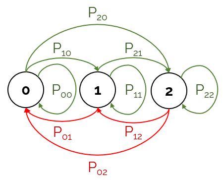
Number of heads cannot decrease; edges in **red** have a value of 0.

We already have the state space of our problem, and now we only need to define the transition probability matrix. A reminder here that $r$ denotes the number of coins. As an example, here’s a visualisation of $P_{4,2}$ :

With this visual representation, we can easily derive the expression:

$P_{ji}={r-i\choose j-i}p^{j-i}(1-p)^(r-j)$

For 6 coins, $P$ will be a 7×7 matrix. The useful property of $P$ is that the probability of transition from state i to state j in t steps is simply $\left(P^t\right)_{ji}$ .

We will now define a State Vector, $s_t$ , which contains 7 components, each being the probability of being in that particular state at step t. Since we start at state 0 with probability 1, our initial state vector is:

$s_0=\begin{pmatrix}1\\0\\0\\0\\0\\0\\0\end{pmatrix}$

We can use the transition probability matrix to get the state vector at any step:

$s_t=P^ts_0$

absorbing states

An Absorbing State is a state in a Markov Chain which transitions to itself with a probability of 1. This means that when our state transitions into an absorbing state, it will remain in that state until the end of time.

Notice that in our problem, once there are 6 heads, we stop flipping any coins. Looking at it in another perspective, this means that any step from state 6 onwards will not change the state. In other words, state 6 is an absorbing state, and thus the expected number of steps we stay in state 6 is infinity.

solving the problem

Now that we have the tools we need, we can tackle the actual problem.

How can we use our initial state vector and transition probability matrix to find the expected number of steps for all coins to land on heads? At step t, the probability of being in state k is the (k+1)^th component of $s_t$ (assuming our components are numbered from 1). If we sum $s_t$ where t goes from 0 to ∞, we get the expected amount of time spent in a particular state. We shall call this vector $x$ .

$x=\sum_{t=0}^\infty s_t$

We can express $s_t$ in terms of $s_0$ and $P$ , and we can factorise $s_0$ since it is independent of t:

$x=\left(\sum_{t=0}^\infty P^t\right)s_0$

Now, notice that the expected number of steps for all coins to land on heads is the expected number of steps spent in all states except 6, i.e. the sum of the components of $x$ except the 7^th component. Since the 7^th component is infinity, it would cause problems in our calculation, and we can remove it to get $\hat{x}$ . We would then need to make the following modifications:

Transition Probability Matrix: Remove the 7^th row of $P$ . Since the 7^th column will be left with zeros, remove it as well. We will get a 6×6 matrix $\hat{P}$ .
State Vector: Since we removed the 7^th column of $P$ , we need to remove the 7^th component of $s_0$ . We will get a 6-dim vector $\hat{s}_0$ .

Our equation then becomes:

$\hat{x}=\left(\sum_{t=0}^\infty \hat{P}^t\right)\hat{s}_0$

Now, we have a rather problematic term: $\sum_{t=0}^\infty \hat{P}^t$ . This term only converges if $\hat{P}$ is a Negative Definite matrix. In our case, since we got rid of the last row and column, it happens to be negative definite (proof is left as an exercise to the reader). Let’s denote the result of this sum as $V$ . We can solve for $V$ as follows:

$V=I+\hat{P}+\hat{P}^2+\hat{P}^3+\cdots$

$V=I+\hat{P}\left(I+\hat{P}^2+\cdots\right)$

$V=I+\hat{P}V$

$V=\left(I-\hat{P}\right)^{-1}$

This looks very similar to the formula for the geometric series, because it’s the matrix equivalent. This matrix only exists if there is an absorbing state (or absorbing cycle). There is an interesting physical meaning to each component: $V_{ji}$ is the expected number of steps spent in state j assuming we started from state i. Now, we can substitute this expression back into the original equation:

$\hat{x}=\left(I-\hat{P}\right)^{-1}\hat{s}_0$

Now, only need to solve this equation, and sum the components of $\hat{x}$ . Since $I-\hat{P}$ is lower triangular, the time-complexity is $O(r^2)$ .

Python script:

import numpy as np
from scipy.special import comb
# from math import comb # you can use this instead for Python 3.8+

def generate_P(p: float, num_coins: int):
  return np.asarray([[comb(num_coins-i,j-i) * p**(j-i) * (1-p)**(num_coins-j) for j in range(num_coins)] for i in range(num_coins)]).T

P = generate_P(.5, 6)

print(sum(np.linalg.solve(np.identity(6)-P,[1,0,0,0,0,0])))

Output:

4.034818228366615

simulating it

Of course, no probabilistic write-up is complete without a stochastic simulation. I ran a simulation of 100,000 rounds of coin flips.

Python script:

import numpy as np

def gen_coin_game(p: float, num_coins: int):
  steps = 0
  while num_coins > 0:
    num_coins -= np.random.binomial(num_coins, p)
    steps += 1
  return steps

results = [gen_coin_game(.5, 6) for i in range(100000)]

print('Mean:', np.mean(results))
print('Std:', np.std(results))

Output:

Mean: 4.03891
Std: 1.7926059276650848

Seems to agree well with the theoretical result… or does it?

Exercise: Calculate the p-value of observing this result. With 95% confidence, is the difference from the theoretical value statistically significant?

summary

There is a really neat equivalence between both techniques that were mentioned. If you were observant, you may have noticed that the matrix $A$ from the classic approach and the matrix $\hat{P}$ from the Markov Chain approach have the exact same values, only with a different placement. However, it might not have been apparent in the classic approach that the components of $A$ have the same physical meaning as those in $\hat{P}$ .

representing the coins’ state

the classic way

linear algebra

the engineering way

absorbing states

solving the problem

simulating it

summary

Share this:

Related

Leave a comment Cancel reply