Markovian Russian Roulette

Imagine you are playing a game of Russian Roulette. This game is played, of course, with a revolver:

There are $n$ players.
There are $b$ bullets in the cylinder.
There are $o$ empty chambers in the cylinder (i.e. $b+o$ chambers total).

At the start of the round, the bullets are loaded in a random order with unknown distribution, and the cylinder is cycled. The players then take turns firing the revolver.

If the firing pin strikes an empty chamber, the player succeeds in the current turn, and the next player fires the revolver in the next turn.
When the firing pin strikes a bullet, the game ends with the current player’s loss.

Now, a simple riddle. Assume that you are one of 2 players, and there are 3 bullets + 3 empty chambers. Should you start first or second to have a higher chance of winning?

Now of course, if you’re familiar with this blog, you know we don’t check specific situations. Instead, let’s analyse a simpler variant of this problem first.

two-face’s gamble

Let’s say our good friend Harvey Dent has come to visit the family for the night. And he wants to play a game with us because we play games with others. He sets the rules as follows:

On every turn, Two-Face flips a biased coin where denotes the probability of heads.
- If it lands heads, the player is spared, and the turn goes to the next player.
- If it lands tails, the player loses, and the game ends.
Players take turns in rotation until someone loses.

Notice that this is essentially the same scenario as the first, except with a twist where the cylinder is cycled between every turn (i.e. probability with replacement). This is equivalent to the case where $p = \frac{b}{b+o}$ .

In this situation, should I start first or second?

markov chain

In this scenario, we have a Markov Chain where heads corresponds to a transition between 2 players. Tails corresponds to a loss of the current player.

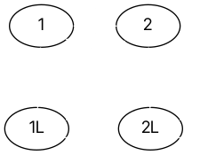
Let’s define our state set with 4 possible states; one for each player, and one for the loss of each player:

$s = \begin{pmatrix}P(1)\\P(2)\\P(1L)\\P(2L)\end{pmatrix}$

And WLOG, we assume Player 1 starts:

$s_0 = \begin{pmatrix}1\\0\\0\\0\end{pmatrix}$

Our transition matrix is:

$P = \begin{pmatrix}0&p&0&0\\p&0&0&0\\1-p&0&1&0\\0&1-p&0&1\end{pmatrix}$

Now, the first thing we want to analyse is the absorption probability of each absorbing state. This means that we are interested in the last 2 components of $s_\infty$ , where:

$s_\infty = P^\infty s_0$

From diagonalisation, we obtain the neat result of:

$s_\infty = \begin{pmatrix}0\\0\\\frac{1}{p+1}\\\frac{p}{p+1}\end{pmatrix}$

observations

Notice first, that:

$\forall p \in [0,1]: \dfrac{1}{p+1} \geq \dfrac{p}{p+1}$

This means that Player 2 always stands a better chance at winning. This, of course, makes intuitive sense, since the probability of losing does not change over time, so it’s always more risky for the one starting first.

Notice also that as $p$ (probability of heads) increases, Player 1 stands a better chance at winning. This also makes intuitive sense.

results

For $n=2,b=3,o=3$ :

$\bar{s}_\infty = \begin{pmatrix}\frac{2}{3}\\\frac{1}{3}\end{pmatrix}$

For neatness, the leading zeros are not included. Player 1 has a 66.7% chance of losing.

russian roulette

Now let’s look at the original scenario. Our Markov Chain used in the variant can no longer work, because the later we are in the game, the higher the chance of firing.

Notice also that by the pigeonhole principle, there is a hard limit on the number of turns. The maximum number of turns that can elapse before someone loses is equal to the number of empty chambers. Once all empty chambers are struck, the next strike will definitely hit a bullet.